Boston Housing Kaggle Challenge with Linear Regression
Boston Housing Data
The database is kept by Carnegie Mellon University and was obtained from the StatLib library. The housing costs in Boston are the subject of this dataset. There are 506 instances and 13 features in the supplied dataset.
The following table shows the summary of the dataset, which was derived from the citation below. Our goal is to develop a model with this data utilizing linear regression to forecast the price of homes.
The following columns are present in the data:
- Crime rate by town, expressed as "crim."
- percentage of residential land that is zoned for lots larger than 25,000 square feet.
- The percentage of non-retail business acres per town is called "indus."
- Charles River dummy variable (= 1 if the tract boundaries the river; 0 otherwise) is called "Chas".
- nitrogen oxides concentration: "nox" (parts per 10 million).
- "rm" stands for "rooms per house on average."
- Age: the percentage of owner-occupied homes constructed before 1940.
- weighted average of the travel times to five Boston employment hubs is "dis."
- "rad" stands for the accessibility index for radial highways.
- Property tax calculated at the full value rate per $10,000.
- Pupil-teacher ratios by town, or 'ptratio'
- "Black": 1000(Bk - 0.63), where Bk is the share of black people in each town.
- "lstat" stands for the population's lower status (percent).
P.S. I am still learning how and where to interpret the graphs; this is my first analysis.
Code:
- import pandas as pd
- import numpy as np
- #importing the libraries
- import matplotlib.pyplot as plt
- import seaborn as sns
- %matplotlib inline
- # Bringing in DataSet and Examining Data
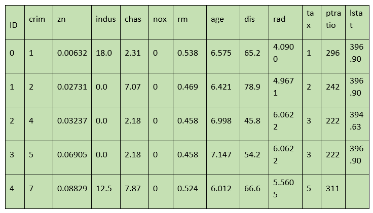
- BostonTrain_in = pd.read_csv("../input/boston_train.csv")
- BostonTrain_in.head()
Output:
Input:
- bostonTrain_in.data.shape
Output:
Input:
- bostonTrain_in.feature_names
Output:
Array[ 'crim', 'zn', 'indus' ,'chas', 'nox' , 'rm', 'age', 'dis', 'rad', 'tax', 'ptratio' ]
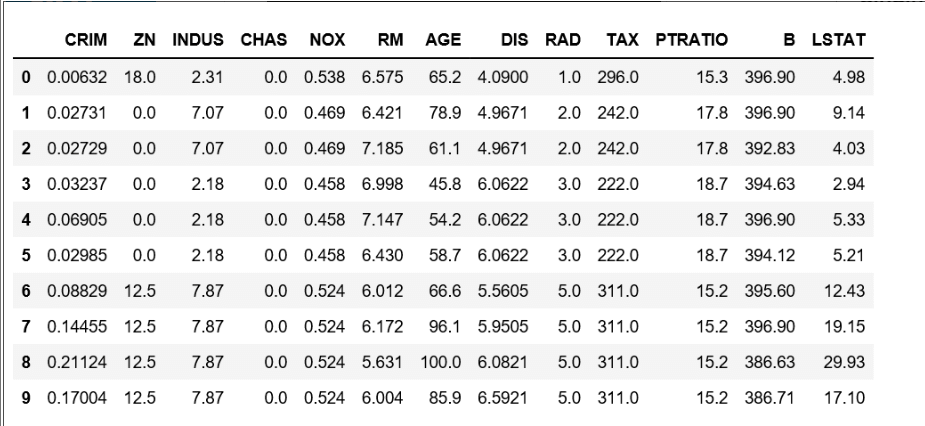
Data conversion to nd-array to info frame and feature names addition
Input:
- data = pd.DataFrame(bostonTrain_in.data)
- data.columns = bostonTrain_in.feature_names
- data.head(10)
Output:
Input:
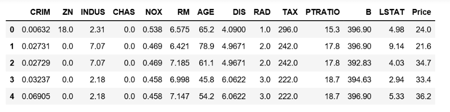
- # increasing the data's "Price" (goal) column
- bostonTrain_in.target.shape
Output:
Input:
- data['Price'] = bostonTrain_in.target
- data.head()
Output:
Obtaining input and output data, then dividing the data into training and testing datasets.
- # Input in the Data
- a = boston.data
- # Output of Data
- b = boston.target
- # dividing the dataset into a training and test set.
- # the submodule cross validation has been renamed and deprecated to model selection from sklearn.cross validation import train test split
- from sklearn.model_selection import train_test_split
- atrain, atest, btrain, btest = train_test_split(a, b, test_size =0.2, random_state = 0)
- print("atrain shape flow : ", atrain.shape)
- print("atest shape flow : ", atest.shape)
- print("btrain shape flow : ", btrain.shape)
- print("btest shape flow : ", btest.shape)
Output:
atrain shape flow: (403, 13)
  atest shape flow: (102, 13)
  btrain shape flow: (404, )
  btest shape flow: (102, )
utilising the dataset and a linear regression model to anticipate prices.
- # Multilinear regression model fitting to training model
- from sklearn.linear_model import LinearRegression
- reg = LinearRegression()
- reg.fit(atrain, btrain)
-
- # predicting up the test set of results
- b_pred = reg.predict(atest)
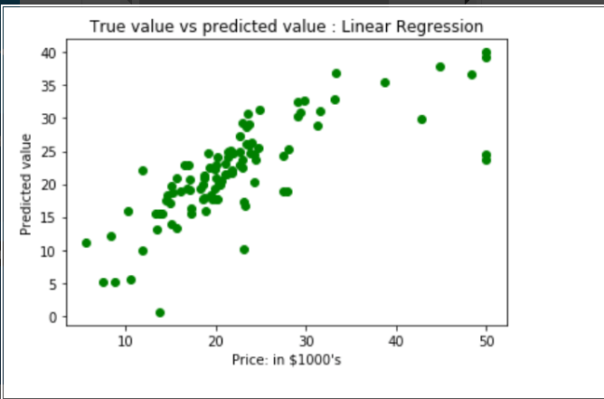
Plotting a scatter graph to display the 'y true' value vs 'y pred' value will show the prediction results.
- # Plotting a scatter graph to display the results of the prediction (btrue vs. b pred)
- plt.scatter(btest, b_pred, c = 'green')
- plt.alabel("Price: in $1000's")
- plt.blabel("Predicted value")
- plt.title("Linear Regression: True value versus forecasted value ")
- plt.show()
Output:
Mean Squared Error & Mean Absolute Error are the results of linear regression.
- from sklearn.metrics import mean_square_in_error, mean_absolute_in_error
- m1 = mean_squared_error(btest, b_pred)
- m2 = mean_absolute_error(btest,b_pred)
- print("Mean Square Error is : ", m1)
- print("Mean Absolute Error is : ", m2)
Output:
Mean Square Error is :  33.4489799151161496
  Mean Absolute Error is :  3.8429092484151966
As a result, the accuracy of our model is just 66.55%. The prepared model is therefore not particularly effective in forecasting home prices. Using a wide range of additional machine learning methods and approaches, one can enhance the prediction outcomes.
Feedback
- Send your Feedback to nigammishra826@gmail.com
|